Case Study: turbopuffer ANN v3

turbopuffer is all the rage in vector dbs! In the past, its sizing guide recommended against using turbopuffer if the direct search corpus exceeded a certain number of vectors, likely 1B. In other words, it was built more for multi-tenanted/multi-namespaced hosting use cases, such as its current customers, Cursor, Notion, where each tenant/namespace (end user) would only search a very small portion, filtered down to their own data. Lately, it published an article, explaining searching against a 100B-vector corpus at a whopping 1k qps throughput. There were a lot of admirable first-principles estimates that guided their design choices.

I would like to write down a few observations, wiggle a few parameters, and do some cost analyses.

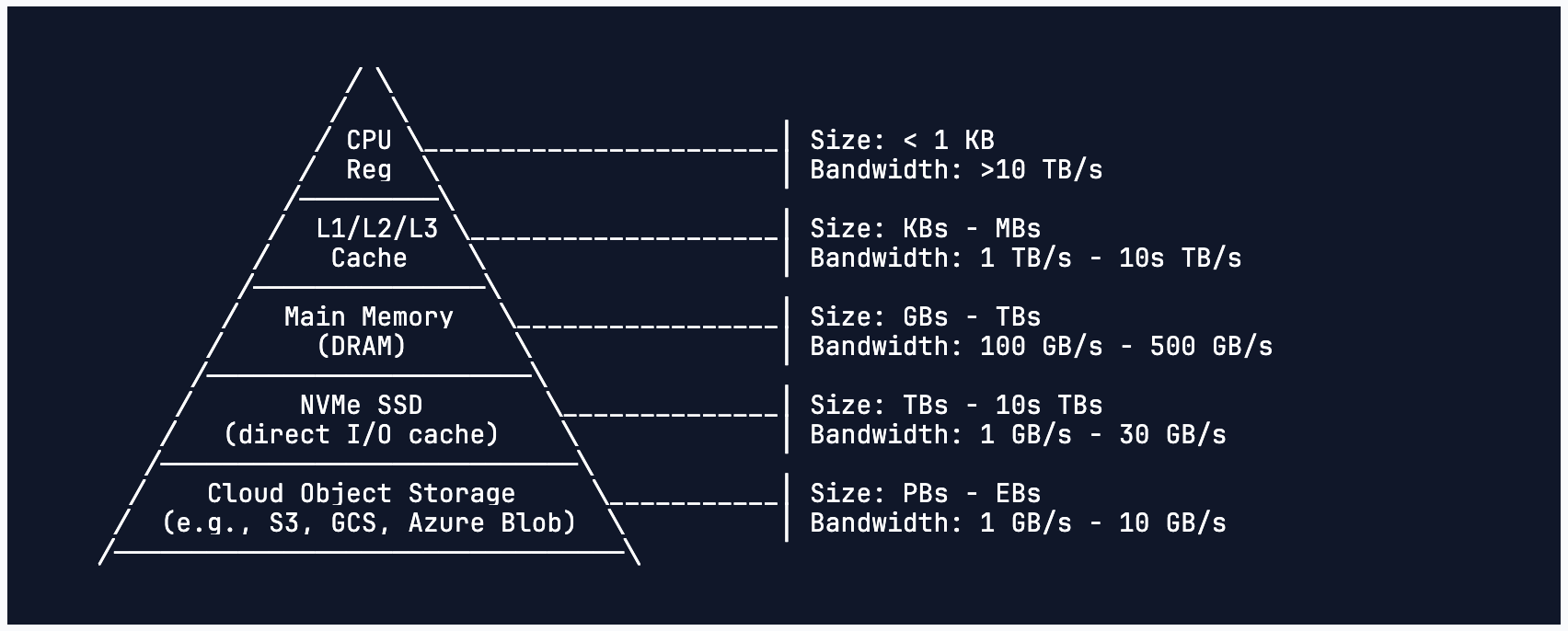
Vector search is a punishing data access pattern - everything is larger. One field is as big as DIM x DTYPE_SIZE bytes, instead of a single INT64, and the entirety of the field is needed in the query hot path. This makes everything downstream constrained by the sheer data quantity, and bandwidth-bound. Traditional databases put smallish indexes in-mem, and do most of the DB operations on disk. In contrast, vector indexes are big, and often need to reside in DRAM entirely to work properly due to graph-like access patterns. Unless filtered down to a brute-force scannable segment by some natural predicate, it usually means a lot of bandwidth and a lot of compute.

Multi-tenanted use cases provide a great opportunity for optimization by amortization, as any large infra/platform/insurance providers would do - pooling uncorrelated demands/risks lets you provision for the average rather than the peak. For example, S3 specialized into a low-cost storage paradigm, based on the right observation that most people store a lot of data, but very infrequently query some of them. If they spread out data in many HDDs, one user’s bursty workload can be spread across many of them through prefixes, thus delivering a lot of throughput, and a decent amount of IOPS. Overall the ecosystem benefits from this specialization.

Vector search over a single large corpus is an even more punishing data access pattern - in theory, the entirety of your corpus needs to be considered. You can’t use the above amortization optimization anymore. As a platform provider, turbopuffer entered into a different race with a new customer profile that wants to search through a single namespace without additional filtering. Now they need to pound-for-pound optimize for those specific customers and make sure their demands are expressed with the best tradeoffs. These customers could make different choices because they are the consumer of a database that ideally fully serves their needs, instead of the provider of a database that needs to find common ground from a lot of customers. These customers could ask for a lot of optimizations uniquely afforded by them, given their own insights, and have better definitions of acceptable tradeoffs.

Cost at 1k qps

Let’s calculate how much it costs for the final setup to reach 1k qps. At the beginning of the article:

100 billion vectors, 1024 dimensions per vector, 2 bytes per dimension (f16). This is vector search over 200TiB of dense vector data.

And almost at the end:

The lowest level of the quantized ANN tree is stored in DRAM, as was the case before. However, because these vectors are compressed, they require less memory bandwidth to access.

This requires 100B x 1024/8 bytes = 12.5TiB of DRAM!

Looking around EC2 instance options, getting 13 x i4i.32xlarge instances (1TiB each) can fulfill the DRAM requirement. Each instance comes with a total of 29TiB NVMe drive space with a RAID0 setup as the disk cache. r6id.32xlarge has the same CPU/DRAM specs, but falls short at only 7.4TiB disk space. i7is are very similar to i4is with better CPUs, but come with a premium. They both support AVX-512. So let’s just use the less aggressive estimate.

With on-demand pricing, it amounts to 13 x $10.98/hr = $142.8/hr ($103k/mo)! With a 3-year savings plan, 13 x $5.08/hr = $66.04/hr ($48k/mo). More than half a mil annually.

But Wait…

In their final setup,

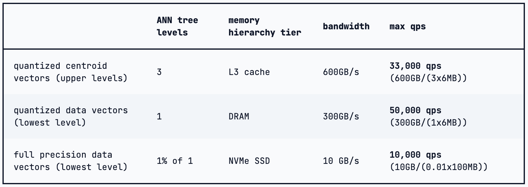
See how the DRAM and NVMe SSDs have so much unused capacity. They explained that the scheme became completely compute-bound with much smaller (f16 -> bit, 1/16) vector sizes. That was true, but that was due to a choice that put all 12.5TiB RaBitQ-quantized vectors into DRAM, and left SSDs only responsible for 1% of the leftover reranking work! There has to be a middle ground somewhere…

I believe there was something off about the estimation method. In the scale chart,

the cloud object storage bandwidth was in line with my past experience on AWS. In fact, AWS would typically rate-limit one IP in the same region from downloading more than 50 Gbps from a single bucket (my Rust-based sulfite downloader would initially go over, but got capped quickly). The NVMe SSD bandwidth was estimated close to what a single i4i.32xlarge with 29TiB would deliver, ~15GB/s. To prove it, I started one and tested it:

--> sudo fio --name=seqread --ioengine=libaio --rw=read --bs=16k --size=1G --numjobs=1024 --runtime=30 --time_based --direct=1 --group_reporting --filename=/mnt/raid/test
seqread: (g=0): rw=read, bs=(R) 16.0KiB-16.0KiB, (W) 16.0KiB-16.0KiB, (T) 16.0KiB-16.0KiB, ioengine=libaio, iodepth=1
...
fio-3.28
Starting 1024 processes
Jobs: 1024 (f=1024): [R(1024)][100.0%][r=14.4GiB/s][r=944k IOPS][eta 00m:00s]
seqread: (groupid=0, jobs=1024): err= 0: pid=18324: Wed Feb  4 23:30:40 2026
  read: IOPS=919k, BW=14.0GiB/s (15.1GB/s)(421GiB/30005msec)
    slat (usec): min=2, max=2766, avg= 7.44, stdev= 5.94
    clat (usec): min=86, max=51355, avg=1103.34, stdev=1026.37
     lat (usec): min=108, max=51368, avg=1110.91, stdev=1027.03

--> sudo fio --name=seqread --ioengine=libaio --rw=read --bs=16k --size=1G --numjobs=1024 --runtime=30 --time_based --direct=1 --group_reporting --filename=/mnt/raid/test
seqread: (g=0): rw=read, bs=(R) 16.0KiB-16.0KiB, (W) 16.0KiB-16.0KiB, (T) 16.0KiB-16.0KiB, ioengine=libaio, iodepth=1
...
fio-3.28
Starting 1024 processes
Jobs: 1024 (f=1024): [R(1024)][100.0%][r=14.4GiB/s][r=944k IOPS][eta 00m:00s]
seqread: (groupid=0, jobs=1024): err= 0: pid=18324: Wed Feb  4 23:30:40 2026
  read: IOPS=919k, BW=14.0GiB/s (15.1GB/s)(421GiB/30005msec)
    slat (usec): min=2, max=2766, avg= 7.44, stdev= 5.94
    clat (usec): min=86, max=51355, avg=1103.34, stdev=1026.37
     lat (usec): min=108, max=51368, avg=1110.91, stdev=1027.03
    clat percentiles (usec):
     |  1.00th=[  204],  5.00th=[  297], 10.00th=[  379], 20.00th=[  490],
     | 30.00th=[  603], 40.00th=[  742], 50.00th=[  881], 60.00th=[ 1037],
     | 70.00th=[ 1270], 80.00th=[ 1565], 90.00th=[ 2073], 95.00th=[ 2507],
     | 99.00th=[ 3556], 99.50th=[ 4293], 99.90th=[14353], 99.95th=[19006],
     | 99.99th=[28705]
   bw (  MiB/s): min= 2841, max=17049, per=100.00%, avg=14370.15, stdev= 2.09, samples=60416
   iops        : min=181572, max=1090402, avg=919380.14, stdev=134.08, samples=60416
  lat (usec)   : 100=0.01%, 250=2.61%, 500=18.59%, 750=19.32%, 1000=17.26%
  lat (msec)   : 2=31.16%, 4=10.44%, 10=0.44%, 20=0.13%, 50=0.04%
  lat (msec)   : 100=0.01%
  cpu          : usr=0.44%, sys=1.20%, ctx=27584225, majf=0, minf=20030
  IO depths    : 1=100.0%, 2=0.0%, 4=0.0%, 8=0.0%, 16=0.0%, 32=0.0%, >=64=0.0%
     submit    : 0=0.0%, 4=100.0%, 8=0.0%, 16=0.0%, 32=0.0%, 64=0.0%, >=64=0.0%
     complete  : 0=0.0%, 4=100.0%, 8=0.0%, 16=0.0%, 32=0.0%, 64=0.0%, >=64=0.0%
     issued rwts: total=27581027,0,0,0 short=0,0,0,0 dropped=0,0,0,0
     latency   : target=0, window=0, percentile=100.00%, depth=1

Run status group 0 (all jobs):
   READ: bw=14.0GiB/s (15.1GB/s), 14.0GiB/s-14.0GiB/s (15.1GB/s-15.1GB/s), io=421GiB (452GB), run=30005-30005msec

Disk stats (read/write):
    md0: ios=27540231/1, merge=0/0, ticks=28944453/0, in_queue=28944453, util=95.65%, aggrios=3447628/0, aggrmerge=0/0, aggrticks=3583264/0, aggrin_queue=3583264, aggrutil=95.15%
  nvme3n1: ios=3462858/0, merge=0/0, ticks=3868512/0, in_queue=3868512, util=95.15%
  nvme6n1: ios=3450333/0, merge=0/0, ticks=4140371/0, in_queue=4140372, util=94.52%
  nvme2n1: ios=3432066/1, merge=0/0, ticks=3686629/0, in_queue=3686630, util=94.43%
  nvme5n1: ios=3453552/0, merge=0/0, ticks=3129646/0, in_queue=3129646, util=94.54%
  nvme8n1: ios=3441541/0, merge=0/0, ticks=3170668/0, in_queue=3170669, util=94.49%
  nvme1n1: ios=3434711/0, merge=0/0, ticks=3979054/0, in_queue=3979055, util=94.45%
  nvme4n1: ios=3458483/0, merge=0/0, ticks=3662792/0, in_queue=3662792, util=94.58%
  nvme7n1: ios=3447483/0, merge=0/0, ticks=3028440/0, in_queue=3028440, util=94.50%

However, with 13 nodes, they cumulatively should stack up to 195GB/s! A balanced SPTAG index should pretty evenly distribute its data to all the SSDs. Now the SSDs look wayyy more over-provisioned. I wouldn’t be surprised if the DRAM and CPU cache numbers needed to be adjusted due to multiplication - dependent upon how their implementation branches off the non-root level centroid vectors.

With all this extra capacity from SSDs, why don’t we just put the RaBitQ-quantized vectors back onto them? A total of 12.5TiB is just chump change compared to the original 200TiB of f16 vectors. With this new estimate, we can use fewer instances. Let’s stick with i4i.32xlarge, and use SSDs instead of DRAM as the constraint, (200TiB + 12.5TiB) / 29TiB = 7.3 -> 8 instances. This just brought down the cost by ~40%. Using the same bandwidth limit estimate for SSDs, we got 8 x 15GB/s = 120GB/s, 120GB/(1x6MB) = 20,000 qps. This is more than enough, still compute-bound.

It even makes their initial setup without RaBitQ quantization work:

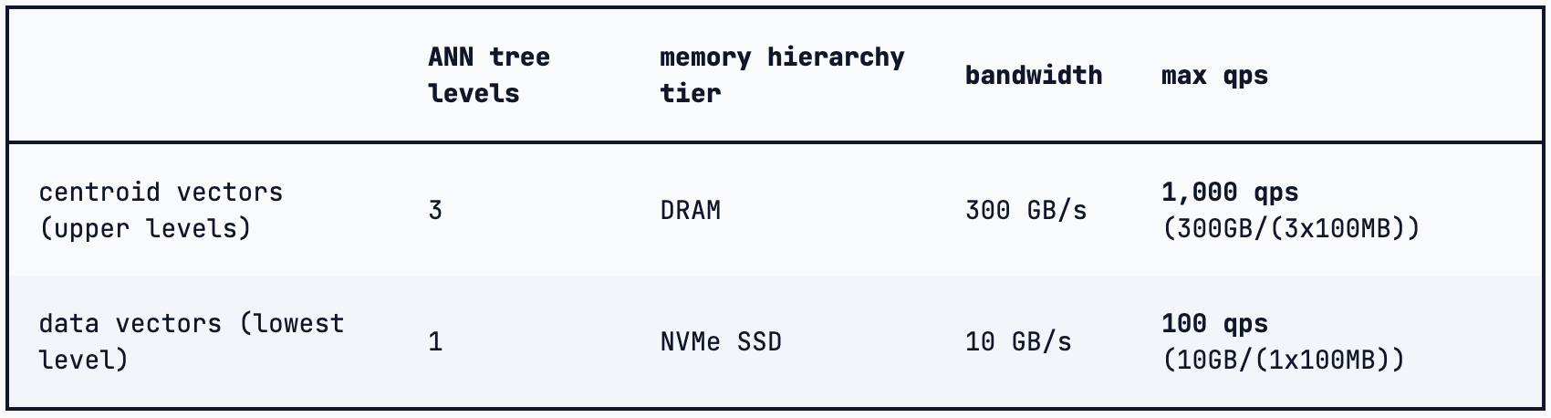
At fp16, 120GB/(1x100MB) = 1,200 qps, just enough to match the target. However, fp16 usually is a lot more compute-intensive than binary calculations. If they got compute-bound 1k qps doing RaBitQ, compute-bound fp16 is going to be a lot slower.

Of course, we miss out on the extra CPUs from the other 5 nodes, and DRAM gets woefully under-utilized. i-family instances have r-family level CPU/DRAM ratio, and over-provision on DRAM. Is there a more CPU heavy instance type with a lot of disks? c6id.32xlarge comes to mind with 128 vCPUs (same as i4i.32xlarge) and 256GB DRAM, instead of 1024GB. But like r6id.32xlarge, they only carry 7.4TiB disk space. (200TiB + 12.5TiB) / 7.4 = 28.7 -> 29 instances! This amounts to a 3-yr savings plan 29 x $2.696/hr = $78/hr, $78 / $66 = 1.2x more than the original budget. However, it is a net more balanced configuration, because you now get to have 29 / 13 = 2.23x more CPUs to solve your compute-bound problem, so the overall qps should multiply as much. This might be what some bigger customers need.

Re-examining the Original Vectors

What’s up with fp16 for original vectors? The industry finally accepted fp32 was too much for vector data, and fp16 wouldn’t cause any significant accuracy loss. Most models are even trained with fp16 autocast on most layers and ops, and the fp16 final embeddings are more than fine for L2 distance/cosine similarity calculations. But what about INT8? In practice, it leads to less than 0.01 accuracy loss. For a well-tuned embedding model (texts or images), the similarity range is wide and clear, <0.4 for dissimilar, 0.4~0.6 for some relevance, and >0.6 for similar. You can totally use INT8 quantization. Best, to preserve more accuracy, use non-uniform scalar quantization so that each dimension gets its own dynamic range trained by representative data. This cuts down your 200TiB original vectors by half! So (100TiB + 12.5TiB) / 7.4 = 15.2 -> 16 c6id.32xlarge instances. 16 x $2.696/hr = $43/hr, $43 / $66 = 65% the original budget, and 16 / 13 = 1.23x more CPUs to run RaBitQ. INT8 also runs faster than fp16 for distance/similarity calculations.

If you go down further to non-uniform INT4, in my setup, the accuracy loss is at max 0.03 by comparing the unquantized query vector to quantized corpus vectors, and 0.06 by comparing two quantized vectors. It might be unacceptable for some, but a great budget option for others. Accepting the loss, INT4 is even faster than INT8. INT6 is a weird one. It’s usually a better trade-off midpoint between INT8 and INT4, but it’s not byte-aligned, so usually slower than INT8. However (many turns in this line of reasoning), if you use RaBitQ, and only use 1% of original vectors to rerank, speed is not an issue here, so just pick your acceptable accuracy-compression tradeoff point. If you do go down to INT4, or somehow find an INT2, there might be no need to keep the RaBitQ quantizer.

Also, maybe your embedding model could be retrained or fine-tuned to use a smaller output dimension with negligible accuracy loss. This is where it helps to optimize the entire ML<>Data as a system, because a decision during training that helped hit leaderboards might come back to haunt you if that means doubling a huge amount of infra cost to store. Study and document it, and you might just get another 1/2 factor! Vector search is full of these 1/2 (or 2x) factors, and when you stack them up, suddenly you get an order of magnitude of differences!

The 100 qps Target

What if I don’t need 1k qps? Let’s re-evaluate the 100 qps target given what we just went through. At this scale, the extra CPUs are extra cost to avoid, so we need to choose a high SSD/CPU ratio instance type. i3en.24xlarge with 96 vCPUs, 768GB DRAM, and 58.5TiB SSDs is great for this. (100TiB + 12.5TiB) / 58.5TiB = 1.9 -> 2 instances. 2 x $4.72/hr = $9.44/hr, $9.44 / $66 = 14% the original budget, and 96 * 2 / 13 / 128 = 12% the original CPU power. Sounds about right.

The Budget Option for 100B

What if you only need 1~10 qps? This is the true budget option. At this scale, the extra speed NVMe SSDs offer is even extra cost to avoid. Should you appreciate the wonder of gp3 EBS drives? Take an r6in.4xlarge (n for high-throughput EBS access), and pair with 2 x 64TB drives, and pay for some extra IOPS and throughput (not counted): $0.565/hr + $0.08/GB/mo * 128000GB / (30 * 24 hrs/mo) = $14.8/hr. That’s already more expensive than the 100 qps target.

In their original blog article, turbopuffer said they built an LSM-tree directly on object storage. That might bring the instance cost down to a fraction of what you pay for object storage, which is roughly (100TiB + 12.5TiB) x $20/mo/TiB / (30 x 24 hrs/mo) = $3.1/hr on AWS S3.

Conclusion

You should be able to get more bang for your buck, by putting quantized vectors onto SSDs, choosing more compute-optimized instance types, and re-examining the original vector precision tradeoffs. Moreover, scaling down from the mighty 1k qps is graceful and elastic. turbopuffer is really cool.